Exercise 1: The Draining Tank

Imagine the following scenario: You have a rectangular tub with an area of 2 ft². In the bottom of the tub is drain with an area of 0.1 ft² (a diameter of roughly 2 inches). You add water at a rate of 1 cubic foot per second (about 8 gallons per second). Find the equilibrium volume of water in the tub by doing performing the following calculations

Calculate the volume of water in the tub at one second intervals by adding the amount added in each interval to the amount present at the beginning of that interval and subtracting the amount lost through the drain. At the very beginning there is no water in the tub so the amount lost is zero. Thus the volume after 1 second is calculated to be:

Vol_1sec = 0 + 1 - 0 = 1

During the second interval we again add 1 ft³ to the 1 ft³ remaining from the first time interval. Now, however, there is water in the tub, so some is lost. The amount of water lost through the drain is given by:

where A = drain area (0.1 ft³)

t = length of time interval (1 sec)

g = acceleration due to gravity (32 ft/sec²)

h = height of water in tub (h = Vol_tub/Area)
 
 

When calculating the height of the water, use the water volume in the tub at the beginning of the time interval, that is, prior to the addition of more water. So, during the second time interval (between 1 and 2 seconds) we use a tub volume of 1 ft³; this gives a drained volume of 0.57 ft³. So the volume after two seconds is

Vol_2sec = 1 + 1 - 0.57 = 1.43 ft³.

Repeat the procedure for the third time interval. You should find that 0.68 ft³ drain and the volume is 1.76 ft³.

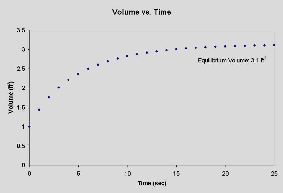
Continue the calculations for several time intervals. Graph the total volume in the tub as a function of time. What does the appearance of the graph say about what is happening physically in the tub? What is happening to the volume lost through the drain in each interval? What does this say about the possibility of reaching equilibrium in the system? Approximately what is the equilibrium volume in the tub?

The "answer":

The above is an example of mathematical modeling: the use of mathematical relationships to calculate, or model, the response of a physical system. All mathematical models share several characteristics. First they all define a specific system, a region in space with defined boundaries. Models attempt to approximate changes that occur within the system boundaries by considering:

initial conditions: the physical parameters of interest at the beginning of a given time frame

inputs: the matter or energy being added to the system; these may be brought in from outside the system or generated internally; in either case, the rate of input must be expressed in the form of one or more equations.

outputs: the matter or energy lost from a system. As in the case of inputs, these can be physically removed from the syste, or may be consumed internally. These must also be expressed as equations.

In the above example, the only variable under consideration was the volume of water in the tub (the system). The input and output were expressed mathematically and the volume was then calculated at regular intervals to determine if equilibrium is ever attained.

A similar approach can be used when calculating what the "expected" temperature of the earth would be in the absence of any greenhouse effect. In this case, the input would be the flux of radiation from the sun. The output would be the earth's blackbody radiation, which will increase at higher temperatures. This example would require more knowledge of the relationship between heat and temperature than we have covered however.

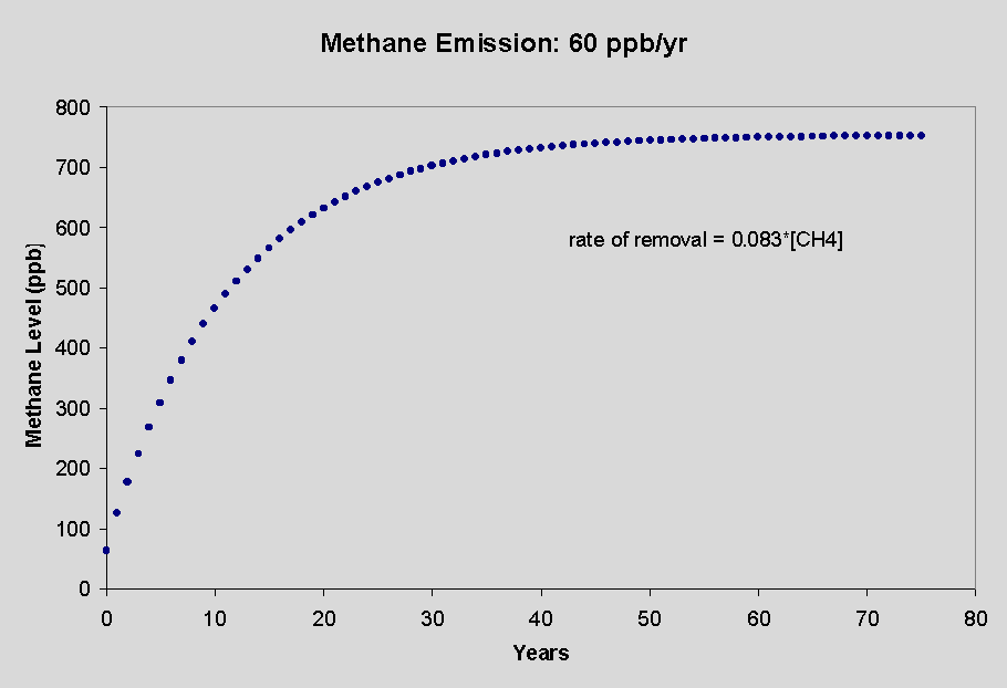
An example that we are prepared to examine has to do with the level of chemical pollutants in the atmosphere. For example, if we are interested in modeling the level methane in the entire atmosphere we can estimate the rate of its emission and removal. The equilibrium methane level is that which is seen when the rate of removal (typically by reaction with hydroxyl radical, × OH) becomes equal to the rate at which it is generated. This is an example of a "zero-dimensional" model because it does not distinguish concentrations spatially or in altitude.
 
 

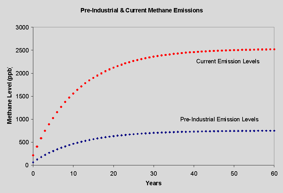
Assuming the we understand the mechanism of methane consumption, we can then use the model to predict what the equilibrium level of methane will be for enhanced rates of generation, such as those that currently exist.

More complex atmospheric models are the so-called one-dimensional models, which give information about the distribution of species with respect to altitude, two-dimensional models, which gives information with respect to altitude and latitude, and three-dimensional models, which give information with respect to altitude, latitude and longitude. Note that all of these models give information with respect to time as well.

Examples of these more complex models are described in your text and are summarized below:

A Two-Dimensional Model: The Effect of Supersonic Aircraft on Stratospheric Ozone Levels in 2015.

initial conditions: estimate of stratospheric ozone levels in the absence of supersonic aircraft in 2015; estimates of other chemical species in the stratosphere.

inputs: calculated exhaust emissions from supersonic aircraft in 2015

Note that these input estimates are, in turn, dependent on the following related estimates: number of flights, emissions expected for a given flight, flight patterns. Other inputs could include chemical reaction products generated within the system

outputs: loss of ozone by known chemical reactions.

A Three Dimensional Model: The Daily Generation of Ozone in the Los Angeles Basin

initial conditions: levels of VOC and other species prior to pre-dawn morning rush hour commutes; physical geography of the basin

inputs: species from automobile exhaust, sunshine, photochemical reaction products including NO₂ and O₃, fresh air blown in from outside the basin

outputs: loss of ozone, polluted air blown out of the basin

Models of Global Warming.

initial conditions: include current levels of greenhouse gases, current weather patterns and mass transport systems, current temperature

inputs: CO₂, CH₄, SO₂, NO₂, CFCs, radiation from the sun

assumptions: economic growth, energy policies, alternative technologies, population growth, economic disparities, environmental regulations

stability of the model:

How will an increase in temperature affect the formation of clouds?
How will warmer oceans affect the carbon cycle? May enhance CO₂ levels.
How will warmer temperatures affect plant life: could affect albedo, carbon cycle
How will warmer temperatures affect relative humidity? could enhance warming
How will warmer air in the arctic affect the thermohaline circulation of ocean water?
 

Given the uncertainties in the underlying assumptions, a variety of scenarios are used to estimate the effects of global warming. A series of such of scenarios have been used by the United Nations to predict the extent of temperature change (see: http://www.ipcc.ch/pub/wg1TARtechsum.pdf). The models project temperature changes between 1° and 3° C by 2050 and between 1.5° and 6° C by 2100.